Earned Value Management: How to Measure and Forecast Cost Performance on Capital Projects

Apr 18, 2026

On a large capital project, it is entirely possible to be within budget at month six and still be heading for a significant cost overrun at completion. Spending is on track — but the work being completed is behind schedule, which means you are paying for time you will never recover. This is the problem that Earned Value Management (EVM) was designed to solve.

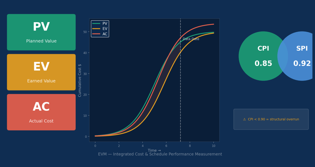
EVM is an integrated cost and schedule performance measurement framework. Rather than comparing what you have spent against a budget, it compares what you have spent against what you have actually accomplished. The difference is fundamental: EVM ties expenditure to physical progress, giving project controls teams a leading indicator of where the project is headed, not just a lagging snapshot of where it has been.

This article covers the core mechanics of EVM — the three baseline metrics, the performance indices, and the key forecasting equations — and explains how to interpret and act on EVM signals in a capital project context.

The Three Pillars: PV, EV, and AC

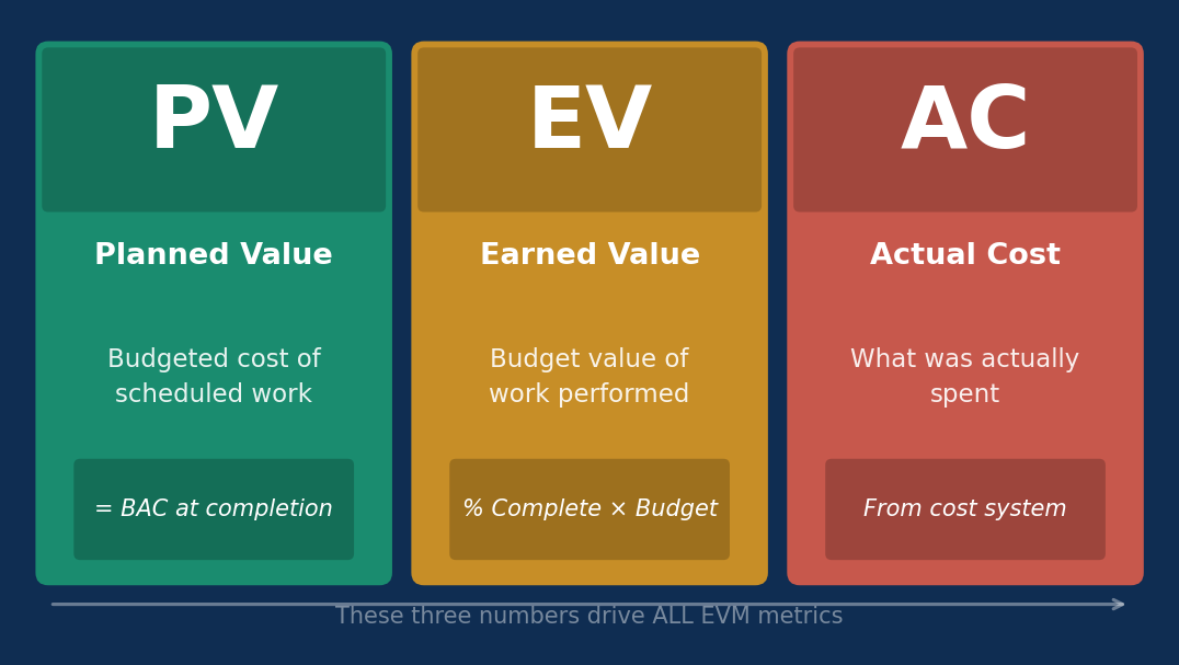
Every EVM calculation is built on three time-phased measurements. Understanding what each one represents — and how it differs from the others — is the foundation for everything that follows.

Planned Value (PV)

Planned Value is the authorised budget assigned to scheduled work at any given point in time. It is derived from the Performance Measurement Baseline (PMB) — the approved, time-phased cost plan. PV answers the question: how much work should have been completed by now, in dollar terms? At project completion, the total PV equals the Budget at Completion (BAC).

Earned Value (EV)

Earned Value is the value of work actually performed, expressed in terms of the approved budget for that work. If you had planned to complete a civil foundation package for $2 million and you have completed 60% of it, your EV for that package is $1.2 million — regardless of what you have actually spent. EV is the key metric in EVM because it links physical progress directly to planned cost.

Actual Cost (AC)

Actual Cost is what you have actually spent to accomplish the work measured by EV. It comes from your cost management system and includes all costs incurred in completing the earned work. The relationship between EV and AC is the core of cost performance measurement.

The three EVM baseline metrics — Planned Value, Earned Value, and Actual Cost — are the foundation of every EVM calculation on capital projects.

Calculating Performance: Variances and Indices

Once you have PV, EV, and AC, two sets of derived metrics tell you how the project is performing on both cost and schedule dimensions.

Metric	Formula	Meaning
CV	EV − AC	Cost Variance: negative means over budget
SV	EV − PV	Schedule Variance: negative means behind schedule
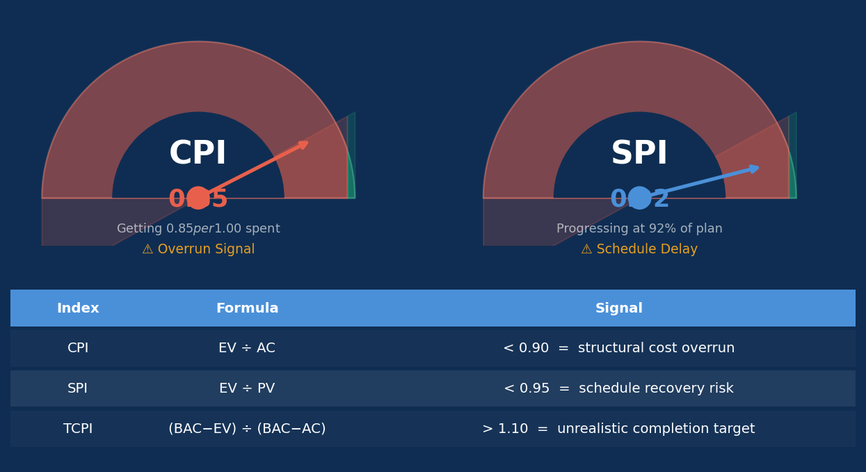
CPI	EV ÷ AC	Cost Performance Index: <1.0 means cost overrun
SPI	EV ÷ PV	Schedule Performance Index: <1.0 means behind plan
TCPI	(BAC − EV) ÷ (BAC − AC)	To-Complete Performance Index: efficiency needed to finish on budget

The indices are more useful than the variances in most reporting contexts because they are dimensionless ratios — you can compare them across work packages of different sizes and track trends over time. A CPI of 0.85 means you are getting $0.85 of earned work for every $1.00 you spend. If that ratio holds, the eventual cost overrun is predictable.

Practical signal: A CPI below 0.90 that persists for three or more reporting periods is a strong indicator that the project’s cost overrun is structural, not a timing anomaly. Research on completed capital projects consistently shows that CPI tends to stabilise after 20–30% of project spend, meaning early signals are meaningful.

CPI and SPI translate raw variance data into dimensionless efficiency ratios that can be tracked across reporting periods to identify structural trends.

Forecasting to Completion: EAC and ETC

EVM’s most powerful application is forecasting — using current performance to predict final project cost. The Estimate at Completion (EAC) answers the critical question: given what we know now, what will this project actually cost?

EAC Methods

There are three common EAC formulas, each encoding a different assumption about how the project will perform for its remaining work:

EAC = AC + (BAC − EV): Future work will be performed at the planned rate. Use this when the cause of the current variance is isolated and corrective action has been taken.
EAC = AC + (BAC − EV) ÷ CPI: Future work will continue at the current cost efficiency. This is the most commonly used formula on capital projects and tends to be the most accurate predictor when CPI has stabilised.
EAC = AC + (BAC − EV) ÷ (CPI × SPI): Both cost and schedule inefficiencies compound. Used when schedule pressure is forcing scope acceleration or overtime that directly increases unit costs.

Estimate to Complete (ETC) and Variance at Completion (VAC)

ETC is simply EAC minus AC — the additional cost required to finish the project. VAC is BAC minus EAC, expressed as the projected cost overrun or underrun at completion. These three numbers — EAC, ETC, and VAC — are the core of any credible monthly cost report on an EVM-enabled project.

Setting Up EVM on a Capital Project

EVM is only as good as the Performance Measurement Baseline it is built on. A weak baseline produces misleading metrics — and on large capital projects, a misleading CPI is worse than no CPI because it creates false confidence.

The Performance Measurement Baseline

The PMB integrates the project scope (via WBS/CBS), schedule (time-phasing), and approved budget. Every work package must have a clearly defined scope, a start and finish date, a budget, and a measurable method for assessing physical progress. Getting this right at the outset is the hardest part of implementing EVM on capital projects.

Measuring Physical Progress

Progress measurement methods vary by work type. Common approaches include: weighted milestones (for discrete, measurable deliverables), percentage complete from an engineering or construction quantity tracker, and level-of-effort for ongoing management activities. The method chosen for each work package should be agreed in the EVM plan before work commences, not estimated retroactively.

Worked Example

Consider a $50 million process plant module. At month 10, the PMB shows PV = $22M. The project team reports EV = $19M and AC = $23M. The resulting metrics are: CPI = 0.83 (EV/AC), SV = −$3M (EV−PV), and SPI = 0.86 (EV/PV). Applying the CPI-based EAC: AC + (BAC−EV)/CPI = $23M + ($31M/0.83) = $23M + $37.3M = $60.3M. The project is tracking $10.3M over its $50M budget, with schedule running at 86% efficiency. That is the signal the project controls team needs to escalate and act on — in month 10, not at handover.

Common EVM Pitfalls on Capital Projects

EVM is frequently implemented but rarely implemented well. The most common failure modes on capital projects are:

Overstated progress: Physical progress is reported optimistically, inflating EV and masking true cost performance. An independent progress verification process is essential, particularly for engineering and construction work packages.
PMB not maintained: Scope changes that are not formally incorporated into the baseline corrupt all downstream metrics. EVM requires rigorous change control — the PMB should be updated only through the approved change process.
Too many level-of-effort work packages: LOE work packages earn value automatically with time, meaning no meaningful cost or schedule signal is generated. Minimise LOE to management and support functions only.
Using SPI without time-based schedule metrics: SPI is a cost-weighted metric and can show a healthy 1.0 even when the project is behind on the critical path. Complement SPI with schedule float analysis and float consumption rates from your scheduling tool.

The three EAC formulas encode different assumptions about future performance — choosing the right one depends on whether the variance is isolated or systemic.

Key Takeaways

EVM integrates scope, schedule, and cost into three metrics — PV, EV, and AC — that together reveal true project performance in a way that budget tracking alone cannot.
CPI and SPI are the most actionable indices: a CPI below 0.90 persisting for multiple periods is a reliable signal of a structural cost problem.
The CPI-based EAC formula — AC + (BAC−EV)/CPI — is the most reliable single-point forecast on capital projects once CPI has stabilised beyond 20% spend.
EVM is only as accurate as the PMB and progress data it is built on. Investment in a well-structured baseline and independent progress verification pays dividends across the full project life cycle.
Complement EVM with qualitative risk intelligence: EVM tells you what is happening; your risk register and schedule analysis tell you why and what comes next.